이원 로지스틱 회귀에 대한 개념설명은 http://statnmath.tistory.com/86 여기 참조하세요~
이번 포스팅은 이원 로지스틱 회귀에 대한 두번째 포스팅으로 모델에 대해 정리해보고자 합니다.
이원 로지스틱 모델은 다음과 같아요.
$Y_{i}|X_{i}$ = 1 if response is in category of interest, 0 otherwise. (Binary!)
where $Y_{i}|X_{i}$ is distributed by Bernoulli ($\pi_{i}$), where $\pi_{i}$ is a probability of success.
즉 일반 선형 모델 (General linear Model)과 다르게 일반화 선형 모델(Generalized Linear Model)이기 때문에 Y값이 continuous하지 않습니다. 이해가 잘 안가시면 그 전 포스팅 참조하세요. 이원 로지스틱이라서 y값이 1 혹은 0을 가지게 되죠. 이때 y는 Bernoulli distribution을 띄기 때문에 y의 평균과 분산 역시 Bernoulli distribution을 따르게 됩니다.
Then $E[Y_{i}|X_{i}]=\pi_{i}$, and $Var[Y_{i}|X_{i}]=\pi_{i} \cdot (1-\pi_{i})$
이원 로지스틱 회귀 조건 중에 참조할 사항으로 분산이 일반 선형 모델과 다르게 일정하지 않다라고 했었죠.
일반화 선형 모델은 선형 모델을 만들어주기 위한 link function이 필요합니다. 그래서 logit과 explanatory variable (X 변수) 가 linear 관계가 되는거죠.
Logistic Regression Model : $log(\frac{\pi}{1-\pi})= \beta_{0}+\beta_{1}X_{1}+...+\beta_{p}X_{p}$
Logistic Function : $\pi=\frac{\exp(\beta_{0}+\beta_{1}X_{1}+...+\beta_{p}X_{p})}{1+\exp(\beta_{0}+\beta_{1}X_{1}+...+\beta_{p}X_{p})}$, where $\exp(\beta_{0}+\beta_{1}X_{1}+...+\beta_{p}X_{p})\in (-\infty, \infty )$
그렇다면 logistic regression model에서 beta값은 어떻게 구할까요? 바로 MLE를 통해 구하게 됩니다.
Data is $Y_{i}$ where 1 if response is in category of interest, 0 otherwise.
Model : $P(Y_{i}=y_{i})=\pi_{i}^{y_{i}}\cdot (1-\pi_{i})^{1-y_{i}}$
Joint Density: $P(Y_{i}=y_{i},...,Y_{n}=y_{n})=\prod_{i=1}^{n}\pi_{i}^{y_{i}}\cdot (1-\pi_{i})^{1-y_{i}}$
where $\pi=\frac{\exp(\beta_{0}+\beta_{1}X_{1}+...+\beta_{p}X_{p})}{1+\exp(\beta_{0}+\beta_{1}X_{1}+...+\beta_{p}X_{p})}$ and $1-\pi_{i}= \frac{1}{1+\exp(\beta_{0}+\beta_{1}X_{1}+...+\beta_{p}X_{p})}$
Joint density 값을 구하기 위해서 데이타 값이 independent해야해요. (서로 결과값에 영향을 미치면 안됩니다.)
Joint Density를 구하면 베타에 대한 likelihood 을 구할 수 있고요~
Likelihood Function will be $L(\beta_{0},...,\beta_{p})= \prod_{i=1}^{n}\pi_{i}(\beta)^{y_{i}}(1-\pi_{i}(\beta))^{1-y_{i}}$
Log 를 씌운 뒤 최대값을 구할 수 있게 되지요. $(\hat{\beta_{0}},...,\hat{\beta_{p}})=\arg \max \left \{ \log L(\beta_{0},...,\beta_{p}) \right \}$
하지만 이 값이 딱 떨어지는 값이 아니게 됩니다. 그래서 Newton-Raphson algorithm 이나 혹은 Fisher Scoring Algorithm을 통해 맥시멈 값을 구하게 됩니다. 물론 컴퓨터가 계산해주죠. 단 한가지 명심해야할 것은, MLE를 통해 구하는거는 데이타 샘플이 충분히 있어야 한다는 점이예요. 그래야 이 beta값이 신뢰할 수 있다라고 합니다. 이해 안가시면 댓글 주세요~
짧게 정리했는데 다음엔 Wald test와 Likelihood Ratio test에 대해 정리해보도록 할게요.
http://statnmath.blogspot.ca/2015/08/the-binary-logistic-regression.html 참고하세요~
[4] Wald Procedure
How can we know whether a explanatory has effect on log-odds or not?
We can use Wald procedure to test whether $\beta's$ are zero or not!!
Hypothesis : $H_{0}:\beta_{j}=0$ which means $X_{j}$ has no effect on log-odds!!, $H_{1}:\beta_{j}\neq 0$
Test Statistics : $Z_{obs}=\frac{\hat{\beta_{j}}}{se(\hat{\beta_{j}})}$
where $\hat{\beta_{j}}$ is a maximum likelihood estimate.
Note that if there is large enough sample, MLE's are normally distributed so that under t$H_{0}$, our test statistics, $Z_{obs}$, is an observation from an approximate Normal(0,1) distribution!!
95% Confidence interval : $\hat{\beta_{j}}\pm 1.96 \cdot se(\hat{\beta_{j}})$
[5] Likelihood Ratio Test
In order to compare which model is appropriate, we can use likelihood ratio test.
Likelihood Ratio : $\frac{L_{R}}{L_{F}}$, where $L_{R}$ is reduced model, and $L_{F}$ is full model of same data.
Hypothesis :
$H_{0}: \beta_{1}=...=\beta_{k}=0$ Reduced model is appropriate so that it fits data as well as full model.
$H_{1}:$ at least one $\beta_{1}=...=\beta_{k}\neq 0$
이원 로지스틱 회귀에 대한 개념설명은 http://statnmath.tistory.com/86 여기 참조하세요~
Test Statistics : $G^2=-2 \log L_{R}-(-2\log L_{F})=-2 \log \frac{L_R}{L_F}$
Note that, under the null hypothesis, $G^2$ is an observation from a chi-square distribution with k degrees of freedom for large n! k is the number of parameter fewer in reduced model.
Remark!! Both Wald Test and Likelihood Ratio Test are testing whether $\beta$ parameter is zero or not! But those two procedures are different so that each following distribution is also different!! Just in case they do not agree, we use the Likelihood Ratio Test since it is more reliable.
'공부정리 > Data Analysis 회귀분석' 카테고리의 다른 글
| Binary logistic regression - 이원 로지스틱 회귀 (4) 예제 Wald Test, Likelihood Ratio Test (0) | 2015.08.17 |
|---|---|
| Binary logistic regression - 이원 로지스틱 회귀 (3) 예제 - 모델과 SAS Code (0) | 2015.08.15 |
| Binary logistic regression - 이원 로지스틱 회귀 (1) - Assumptions (0) | 2015.08.14 |
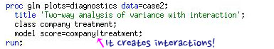
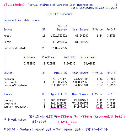
| [SAS] Two Way ANOVA 예제 (0) | 2015.08.13 |
| Two Way ANOVA 개념설명 (0) | 2015.08.12 |