생물학, 통계학, 데이터 과학

http://statnmath.blogspot.ca/2015/08/the-binomial-logistic-regression.html 참고하세요.

Binomial Logistic Regression에서 조건 및 model assessment에 대해 간략히 정리해보려고 합니다.

1. Logit과 X변수간의 linear relationship을 가질것!!

즉, 로지스틱 회귀는 Generalized linear Model인데요. 계속 반복해서 적고 있지만, 일반화선형모델은 Y변수에 변형을 줘서, 즉 link function을 이용해 Y와 X간의 선형적인 관계를 만들어주는걸 말합니다. 그래서 observed logit과 quantitative x 변수간의 scatter plot을 이용해 선형적인 관계인지 확인해야해요.

2. Outlier가 있는지 없는지.

그 전에 정리했던 Binary Logistic Regression은 outlier가 없습니다. 왜냐하면 y값이 어짜피 1 아니면 0 이기때문에 살펴볼 의미가 없었는데요. Binomial Logistic Regression은 binary와 다르게 y값이 카운트 할 수 있어서 outlier의 여부를 살펴봐야합니다.  - 이때 Pearson & Deviance를 통해 outlier의 여부를 알아볼 수 있어요.

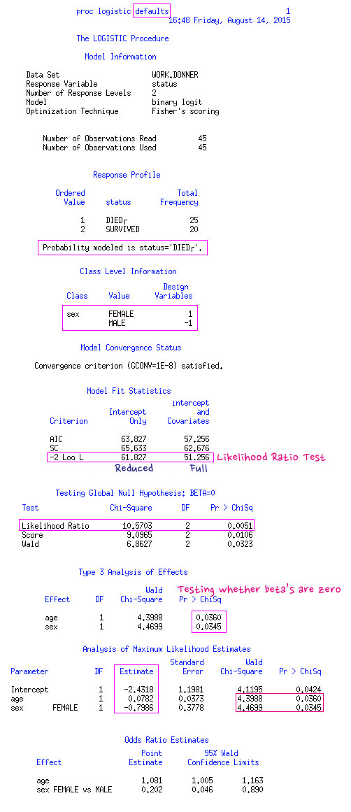
3. Model Fitness - AIC, BIC(SC)

단순한 데이타가 아니라면, 한 데이타 안에서 y값을 설명할 수 있는 식이 여러개 나올 수 있는데요. 그중에서 어떤 모델이 적합한지 알아보려면 AIC, BIC를 이용하면 됩니다.

3.1 Akaike's Information Criterion (AIC)

     AIC = -2 log L + 2(p+1), where 2(p+1) is a penalty and p+1 : # parameters including $\beta_0$

3.2 Schwarz's (Bayesian Information) Criterion (SC)

     SC = -2 logL + (p+1) log N, where (p+1)log N is a penalty and p is the number of explanatory variables

결론은 작은 값이 더 나은 모델을 의미하고요. 특히 AIC값 차이가 10 이상이 난다!! 싶으면 작은 AIC, SC값을 가진 모델이 적합합니다. 그런데 여러 모델의 AIC, SC값 차이가 2 미만이라면 거의 차이 없다라고 생각하면 됩니다.

http://statnmath.blogspot.ca/2015/08/the-binomial-logistic-regression.html 여기 참고하세요.

Binomial logistic regression model (바이노미얼 로지스틱 회귀)은 일반화선형모델의 한 종류입니다. 일반화선형모델은 그 전 포스팅에도 잠시 적었지만, link function을 통해 y변수와 x 변수끼리 선형(linear relationship)을 만들어줍니다. 일반선형모델(General Linear Model)과 다르게 maximum likelihood estimate나 Fisher's scoring을 통해 coefficient of parameters를 구합니다. 그러니까 각 x변수의 계수를 구해서 식을 구해주죠. http://statnmath.tistory.com/81 (일반선형모델에 관한 포스팅) 

[1] Assumptions

Observations are independent, and sample size is large enough for valid inference-tests and confidence interval as the Generalized Linear Model use MLE(Maximum Likelihood Estimate) to predict the parameter coefficients. There is a linear relationship between observed logit and quantitative explanatory variables. 

[2] Model

The response variable is binomial count of the number of "success" Y~ Binomial(m, $\pi$)

$P(Y=y)=\binom{m}{y}\pi^y(1-\pi)^{m-y}$, y=0,1,...,m  

Model: $\log (\frac{\pi}{1-\pi})= f(\mathbb{X}; \beta)$ where $f(\mathbb{X}; \beta)$ is a linear function of the $\beta$'s.

[3] Models and Deviance & Global Likelihood Ratio Test

로지스틱회귀에서 model끼리 비교해볼 수 있는데요. 어떤 모델이 있는지 정리해보자면 크게 세가지가 있습니다. X변수가 X1, X2, X3이 있다고 해요.

3.1 Saturated (Full) Model - 포화모형 : 그러니까 간단하게 생각하면 데이타 자체를 모델화 한거라고 생각하면 됩니다. 즉 y에 대한 식이 X1, X2, X3 이렇게 X변수가 다 들어있습니다. (더 정확하게 설명하려면, X 변수가 있으면 각 X마다 indicator variable로 만들어서 모델을 만듭니다. 이해안가시면 댓글주세요~)

$logit (\hat{\pi})= \hat{\alpha_{0}}+ \hat{\alpha_{1}}I_1+...+ \hat{\alpha}_{n-1}I_{n-1}$

3.2 Fitted (Reduced) Model - 축소모형 : X변수 중 일부만 모형화시킨게 바로 축소모형입니다. 

$logit (\hat{\pi})= \hat{\beta_{0}}+ \hat{\beta_{1}}X$

3.3 Null model - X변수 어떤것도 모델에 반영되지 않는 경우, 즉 Y=bo만 들어있는 식이라고 생각하면 됩니다.

$logit (\hat{\pi})= \hat{\gamma_{0}}$

이렇게 세가지 모델이 있는데 과연 이 모델 중에서 어떤 식이 데이터를 잘 말해줄까...를 고른는거예요.

먼저, Saturated Model과 Reduced Model을 비교하려면, 즉 어떤 model이 더 나은지 비교하려면 Deviance Test를 이용합니다. 

하지만, Reduced Model과 Null Model을 비고하려면 Global Likelihood Ratio Test를 이용합니다.

Deviance Test와 Global Likelihood Ratio Test에 대한 내용은 위의링크 참조하세요. 궁금하신 사항은 댓글주시면 아는 선에서 답변드릴게요~

2.1 Default Code

성별은 categorical variable이어서 class 명령어를 입력하면 여성은 1로, 남성은 -1값으로 설정됩니다. 만약 indicator variable로 만들고 싶다면, 즉 여성은 1, 남성은 0 이렇게요. 그러면 코드를 바꿔주면 되는데 그 전 포스팅에 자세히 적어놓았습니다. 참고하세요~  

2.2 Default  Result

2.3 SAS Result Intepretation 

* Model Equation

$\log(\frac{\hat{\pi}}{1-\hat{\pi}})=-2.43+0.078 \cdot AGE_{i}-0.80\cdot SEX_{i}$

* Wald Procedures(월드검정)

Hypothesis : $H_{0}: \beta_j=0$ vs $H_{1}: \beta_j\neq 0$

Test Statistics: $Z_{obs}=\frac{\hat{\beta_j}}{se(\hat{\beta_j})}$ ~ approx. Normal(0,1) distribution

95% Confidence Interval : $\hat{\beta_j}\pm1.96 \cdot se(\hat{\beta_j})$

월드검정을 통해 나이라는 predictor variable, 그러니까 X 변수가 log-odds 에 영향을 주는지 알아볼 수 있습니다!

Hypothesis: $H_{0}: \beta_{AGE}=0$ vs $H_{1}: \beta_{AGE}\neq 0$

Test Statistics :  $(\frac{-0.078}{0.0373})^2=4.3988$ ~ $\chi_{1}$   

참고로 test statistics이 카이스퀘어 분포를 가집니다. 왜냐하면 Z_obs값이 정규분포 Normal(01,) 에 가깝지만 Z를 제곱한 값은 카이스퀘어 분포를 띄죠.

P-value : 0.036 즉, AGE 변수가 생사여부에 영향을 주네요.

* Likelihood Ratio Test (우도비율검정)

Hypothesis : $H_{0}: \beta_1= \beta_2=0$ vs \H_1$= The Fitted model is better.

Test Statistics: $G^2=-2 \log \frac{L_R}{L_F}=2 \log L_F-2 \log L_R=61.827 - 51.256=10.57$

그러니까 나이와 성별 변수의 coefficient가 0이라면 이 변수가 필요없나는 뜻이겠지요. 그래서 null hypothesis(귀무가설)는 오직 intercept만 필요하다는겁니다. 즉, 나이와 성별 상관 없다는 식이 데이타에 잘 맞는다는 얘기예요. 하지만 alternative hypothesis(대립가설)는 나이와 성별이란 변수가 필요하다!!라는걸 말해요.  

Interpretation : P-value가 0.0051이라서 null hypothesis를 reject 하게 됩니다. 대립가설을 받아드려야하기때문에 fitted model이 더 데이타에 적합합니다. 

Y 염색체 구조에 대해 정리해보겠습니다. 아래 그림처럼 Y염색체에는 male-specific 구역이 있습니다.

Pseudoautosomal (수도오토조멀) is telomeric sequences found on both X and Y chromosomes.  짧은 사슬모양의 중합체로 X와 Y염색체 모두 발견됩니다. 

Y염색체 중에서 male specific 구역은 4개 부분으로 이뤄져있는데요. 1. X-transposed 란 구역은 X염색체와 거의 99% 일치합니다. 2. X-degenerate 부분은 X-linked gene과 60~90% 정도 일치하는 부분이 있고요. 27개 gene 중에 16개는 기능적인 역할이 있고 그중에 SRY gene이 있습니다. 3. Ampliconic는 길고 긴 반복되는 gene으로 되어있고요. 4. Heterochromatic은 tandem이 반복적으로 나타나는 구역입니다.

In male specific region (MSY 95% of Y chromosome) consists of 4 parts; 1) X transposed part which 99% are identical to X chromosome, 2) X-degenerate part which contains genes with 60~96% sequence identify to X-linked genes and 27 genes (only 16 genes are functional) including SRY gene, 3) ampliconic region which is long MSY repeats containing 8 palindromic sequences, and 4) heterochromatic (tandem repeats of low sequence complexity)

palindromes (회문)은 저번에도 설명했지만 앞으로 읽어도 뒤로 읽어도 똑같은걸 말합니다. 만약 GGTACC라는 sequence가 있다고 하면 complementary strand 역시 CCATGG이겠지요. 그래서 만약 복제과정에서 문제가 생긴다면 헤어핀 모양처럼 만들어져서 알아서 고쳐지게 됩니다. 이걸 gene conversion이라고 부르는데 한국말로는 뭐라 부르는지는 모르겠네요ㅠ

In terms of palindromes, Y chromosome contains stretches of DNA in such identical mirror copies of each other. If one of these section makes a hairpin bend in the middle, it appears capable of donating an intact gene to fix a defective copy on the neighboring section. So the Y chromosome seems to have its own self-repair mechanism, a process called gene conversion, maintaining the integrity of the genes without crossover.

Deletion in regions of Y chromosome lead to female or to infertile in males, sometimes there will not affect. SRY gene found near pseudoautosomal region is needed for male determination. In normal exchange between X and Y chromosomes in pseudoautosomal region, it becomes normal female. However, regarding abnormal exchanging between X and Y chromosomes outside of pseudoautosomal region, If SRY male specific gene is relocated onto X chromosome, then this individual become phenotypic male with XX genotype.

Reference: http://universe-review.ca/R11-14-Ychromosome.htm 정말 잘 정리되어있습니다. GOOOOD!!

이원 로지스틱 개념 http://statnmath.tistory.com/86 및 모델 http://statnmath.tistory.com/87 은 링크 참조하세요.

이번 포스팅은 이원 로지스틱 회귀 예제를 들어 정리해보려고 합니다. 자세한 내용은 아래 링크 참조하세요.

http://statnmath.blogspot.ca/2015/08/case-study-binary-logistic-regression.html

Case Study: The Donner Party

Donner와 Reed 가족 87명이 웨건(마차같은거요~)을 타고 이동하는 도중 눈태풍에 갇히게 됩니다. 다음 해 봄, 40명만 구조되었는데요. 나이와 성별, 그리고 생사여부로 데이타가 이뤄집니다.  

2.1. Default Code

먼저 SAS Code에 대해 정리해보겠습니다. proc logistic으로 해서 결과값을 구할 수 있는데요. 문제는 기본적으로 알파벳 순서로 되어있습니다. 즉, Y값이 survival, die로 되어있는데 알파벳 순서라면 die가 먼저 오겠죠. 그래서 die값이 default로 됩니다. 이렇게 프로그램을 돌리면 $\pi$=P(DIE)! 을 기준으로 결과값이 나옵니다.

그리고 성별은 categorical variable이기 때문에 class 명령어를 이용하여 여성과 남성이 각가 1과 -1로 구분하도록 합니다.

2.2. SAS Code - DESCENDING Options

그런데 $\pi$=P(Survival)! 로 하고싶으면 DESCENDING을 입력하면 됩니다.

2.3. SAS Code - CLASS Options

마지막으로 성별을 1과 -1로 코딩하지 않고 indicator variable로 표현하고 싶으면 / param=ref; 명령어를 넣어줍니다. 그러면  $I_{Female}=1$ 여성일 경우, 0은 남성일 경우로 표현됩니다.   

다음 포스팅에서 Wald Test와 Likelihood Ratio Test에 대해 정리해보도록 하겠습니다.